When we talk about analyzing data we usually mean 'doing statistics' but it's always wise to evaluate your findings before you do any formal statistical analysis. For that reason we suggest the following steps when you have some data ready to analyze:
- Plot the data. If you are comparing averages between categories, a box plot, or points with error bars, concisely displace means and variability within each group. If you are comparing two continuous variables (correlation, regression) a scatter plot is an effective visual. If you want to see how data is distributions, use a histogram. Count data is often shown with a bar graph.
- Evaluate the pattern by visually examining the plot and assessing whether there is a strong or weak pattern. Consider whether the differences between means is likely to be biologically important. Does the independent (predictor, x-axis) variable have a strong effect on the dependent (response, y-axis) variable? Does the data appear to be normally distributed?
- Perform the appropriate statistical analysis to answer the question of interest. See below for a simple guide to performing statistical analyses.
- Interpret your results in light of Step 2 and Step 3. The P-value and/or confidence limits will give you some indication of the confidence you should have in the magnitude of the effects that you could see when you evaluated the pattern (Step 2). By convention, when P≤0.05 we say that the results are statistically significant, and thus that we have reasonably good confidence that the size of the effect that we see is reasonably accurate. This does not mean that the effect is biologically (or economically, or medically) significant; that is for you to decide.
Worked Examples
Below we provide simple biological examples that walk you through some of the the steps listed above to give you a better idea as to what we are talking about.
Some Simple Statistical Tests
Below we provide some details and resources on how to perform and interpret the results of some simple statistical tests.
Descriptive Statistics
We use statistics both to describe a sample and to compare samples to one another (e.g., two and multi-sample tests, correlation, regression). There are lots of descriptive statistics but the two that are most generally useful are the mean and confidence limits and we would suggest reporting these two whenever you describe a sample. For continuous data the usual descriptive statistics are:
- Measures of Central Tendency: Mean (arithmetic geometric harmonic), Median, Mode
- Measures of Dispersion: Range, Standard deviation, Coefficient of variation, Percentile, Interquartile range
- Measures of Shape: Variance, Skewness, Kurtosis, Moments, L-moments
Here are some websites for calculating descriptive stats:
- Calculator Soup: using a variety of formats, enter from the keyboard or copy and paste up to 2500 samples; provides details on how each statistic was calculated but does not calculate confidence limits
- Xuru's website: copy/paste data into a box, and get lots of useful descriptive stats including confidence limits of mean and SD
- Graphpad: enter (up to 50 data points) or copy/paste up to 10000 data points or just enter mean and SD to get a few descriptive stats including confidence limits
- HyperStat: basic descriptive stats with stem and leaf display, no CLs
- Had2Know: some unusual descriptive stats (in addition to the usual ones) with good explanations but no CLs
A Worked Example
Dr. Bruce Tufts caught 48 adult Walleye during the spawning season in Lake Nipissing and measured their fork length (a measure of total length in fish). Here are the descriptive stats for that sample:
Parameter | Value |
|---|---|
Mean | 391.91667 |
SD | 49.52791 |
SEM | 7.14874 |
N | 48 |
90% CI | 379.92161 to 403.91173 |
95% CI | 377.53526 to 406.29807 |
99% CI | 372.72548 to 411.10785 |
Minimum | 288 |
Median | 395.5 |
Maximum | 479 |
The 95%CL of the mean tells him that the real mean size of spawning fish in this population is likely to be somewhere between 378 and 406 cm.
Confidence Limits
Confidence limits (CL) provide a way to describe the accuracy of an estimate. Remember that your sample is used to make some inference about the population from which it was drawn. Thus the confidence limits of the mean calculated from your sample tell you the region where the true mean of the population is likely to be. If the CL is large then you do not have much confidence in the true value of the population mean; when the CL is small then you know that the true mean lies within a small range of values.
Strictly speaking, if you were to take 100 random samples from the same population, the 95%CL of 95 of those samples would include the true mean of the population.
When comparing two or more samples, you can use the 95%CL to estimate whether the means are different. If the 95%CLs do not overlap then the true means are very likely to be different and the magnitude of those differences can be anywhere in the range of CLs.
If you know the mean and standard deviation of a sample you can calculate the 95%CL of that mean. To calculate descriptive stats including CL (also called confidence interval, or CI) from raw data you can enter your data and do those calculations. You can also calculate the CL of a proportion.
You can actually calculate the CL for any statistic (SD, correlation coefficient, regression slope, median etc). Wikipedia provides the general principles for calculating CLs.
A Worked Example
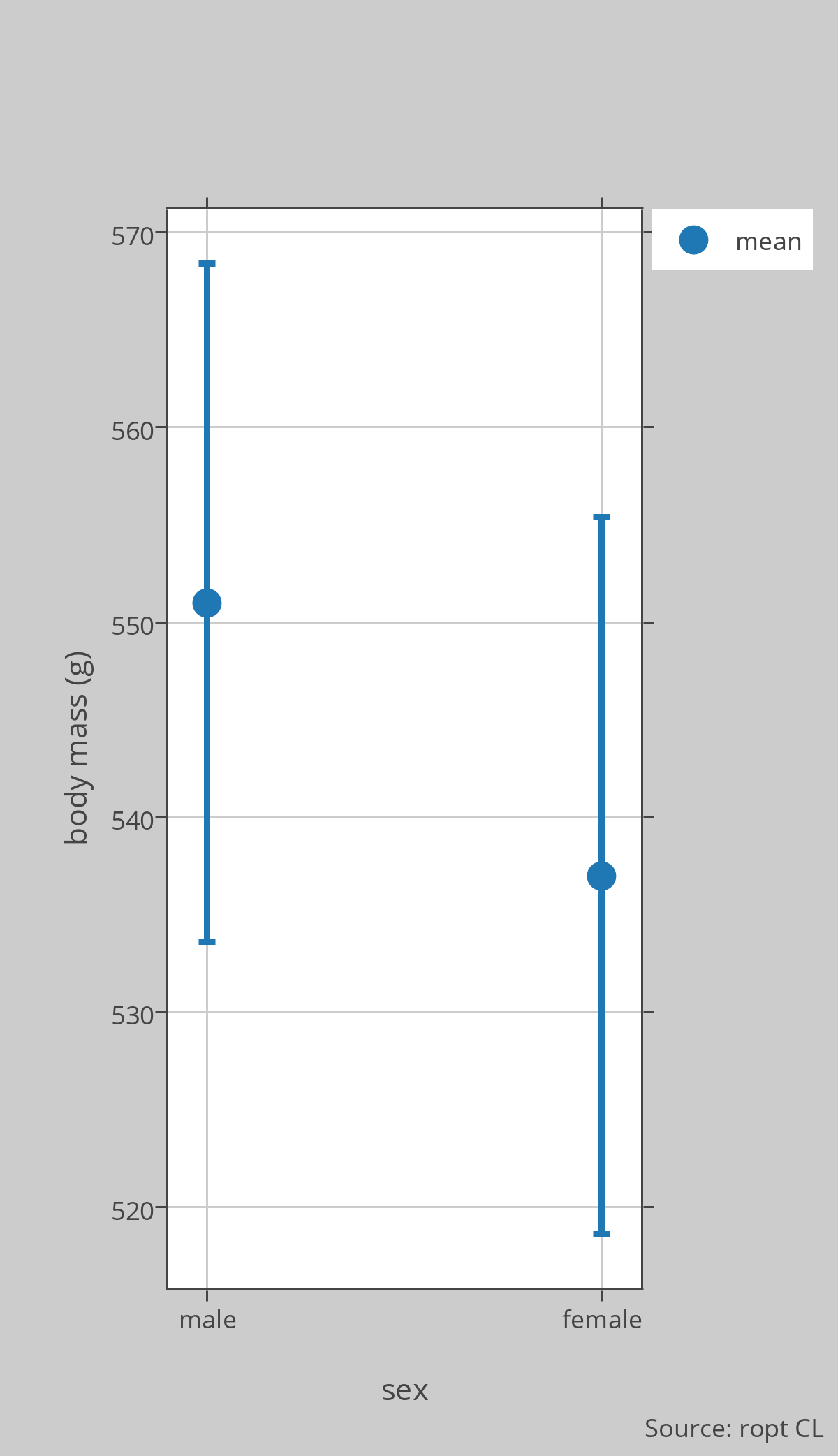
Dr Montgomerie is studying rock ptarmigan at Sarcpa Lake on the Melville Peninsula in the Canadian High Arctic. He is interested in sexual size dimorphism so he caught 10 males and 9 females in June and weighed them. [Note that this is a convenience or volunteer sample, as he just caught true birds he encountered and some birds in this population were too wary to be caught]. The birds weighed, in grams: Males = 620, 600, 597, 520, 585, 570, 585, 540, 545, 570; Females = 550, 540, 545, 510, 530, 585, 525, 520, 530. The descriptive stats, mean [95%CL], are: Males = 551 [534.0–568.4], Females = 537 [519.1–555.4]. The plot in the figure shows the means and 95%CLs.
From this analysis, he can conclude that this sample of males weighed on average about 14g more than the females, but because the 95%CLs overlap, he does not have much confidence in that estimate, nor does he even have much confidence that males actually weigh more than females. The real mean value for males could, for example, be 536g and for females 546g, since those numbers are within the 95%CL of each group. Note that the actual value for males could be even less than 534g and for females even more than 555g, but we are using the 95%CLs here as a guide to the likely values.
Using some fancy stats (power analysis) he figured out that a sample of 25 birds of each sex would be needed to detect a real effect here. He went and caught enough additional birds to bring the sample size to 25 of each sex, and found: Males = 560.4 [551.3–569.5], Females = 542.2 [534.5–549.9]. Now he can conclude with some confidence that males weigh more than females, because the 95%CLs do not overlap, and, based on this sample, that males weigh, on average, 18.2g more than females. It is always possible that this conclusion is wrong (stats are based on probabilities) but this is a reasonable conclusion from the data obtained so far.

Two-Sample Comparisons
To compare the means of two samples, the t-test is usually employed unless the data are ranks, or are so far from normally distributed that you are nervous about the validity of the analysis. To do a t-test, you can use an on-line tool that allows you to enter
- Either your raw data or descriptive stats calculated from those data.
- Just the descriptive stats.
- Just the raw data.
Note that there are lots of options for doing a t-test, depending upon whether you have equal variances or paired data, and whether you want a 1-tailed test or a 2-tailed test. You can learn more about these options here. When in doubt, assume equal variances and unpaired data, and calculate the 2-tailed test.
A Worked Example
Using the example from the Confidence Limits section above, we can compare the weights of male and female ptarmigan using a t-test. For the first sample of 19 birds, the results from the t-test are t = 1.18, P = 0.25, n = 10 males, 9 females. From this analysis you would report: “males weighed 14g, on average, more than females but the difference is not statistically significant (t = 1.18, P = 0.25, n = 10 males, 9 females)”.
Note that sometimes you will get a statistically significant result even when the 95%CLs overlap, but if they do not overlap, then the difference is always statistically significant at P≤0.05.
Multi-Sample Comparisons
The usual way to compare the means of more than two samples (or even just two samples) is with analysis of variance (ANOVA). Just like for the t-test, simple ANOVAs can be performed online:
Most of those sites provide additional useful information about ANOVAs. The most important requirements are that your samples are independent, and that the variances of each sample are similar (the smallest SD should be more than half the largest SD of your samples).
When you run an ANOVA you get and need to report F, P, and two separate degrees of freedom (often called numerator and denominator df). When P≤0.05 we say that the ANOVA is statistically significant and that means only that the means of at least 2 of the samples that you are comparing are significantly different. To find out which pairs of means are different you will need to perform a post hoc test (Tukey HD test is a popular one).
A Worked Example
Dr. Chris Eckert wants to compare the size of flowers in different populations of the beach dune plant Camissoniopsis cheiranthifolia along the cost of California. To do this he haphazardly sampled many plants in each of four populations and measured the width of the corolla, in mm, from one flower on each plant.

Here's a plot of his results, with box plots in red, and the mean and 95%CL of the mean for each sample in green:
He then ran an ANOVA to compare the mean corolla widths and got F = 242.2, df = 4, 518, P<0.0001. Note that there are two different dfs for the ANOVA, the first one (4 here) is often called the among groups df and the second (518 here) the within-groups or error df.
He correctly interprets this as meaning that at least two of the populations have flowers of significantly different size, but he needs to run a post hoc analysis to find which populations are actually significantly different. We can see from the graph, though, and what we know about confidence limits, that there may be more than one pair of populations that have different means. Some caution is needed here because you can't reliably use confidence limits for multiple comparisons.
Nonetheless, the Tukey HSD post hoc tests shows that each mean is significantly different from all of the others:
Note that it is only valid to run a post hoc test if the overall ANOVA is significant, as it is in this example, and that there are no reliable P-values for this test—the differences are either significant or they are not.
Correlation and Regression
Correlation and regression analyses are used to determine how much of the variation in one variable is explained by variation in the other (correlation), and how to predict one variable (the response) from the other (predictor) using an equation (regression). These are two of the most widely used statical analyses in biology. The basic assumptions of these analyses are that the response and predictor variables are normally distributed, and that the relation between them is linear (falls along a straight line). When the correlation coefficient (r is large (close to -1.0 or +1.0) then we say the correlation is strong and thus that the prediction of the response from the predictor is quite accurate. When the slope of the regression line is 1.0 then each increment in the predictor results in an equal increment in the response. Usually correlation and regression analyses are run simultaneously, and it would be unusual to report the regression results without the correlation results. Correlation results often appear alone, however, because we may not be interested in actually making a prediction or knowing the functional relation (slope) between the two variables.
To perform these analyses online you can enter your raw data into one of several tools:
- For lots of detailed output and even some graphs.
- For a simple regression calculator that gives minimal output (with no correlation) and a simple graph (enter data with one sample per line, x then y separated by a space).
- For some really nice output and detailed explanations for both regression and correlation:
A Worked Example
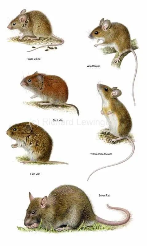
Dr. Chris Moyes has measured the body mass and COX enzyme activity in a sample of individuals from 12 species of small mammals. He calculated the mean body mass and enzyme activity for each species, and log-transformed both variables to make the distributions closer to normal. He then ran a correlation and a regression analysis and got the following results:
- r = -0.72 (P = 0.009)
- a = -0.01 (P = 0.85)
- b = -0.16 (P = 0.009)
Where r is the correlation coefficient and can vary between -1 and +1, a is the intercept of the regression line, and b is the slope of that line. The P-values tell us that r and b are significantly different from zero (note that both always have the same P), and that the intercept is not significantly different from zero, where P≤0.05 is considered to be statistically significant.
You can see from the graph (and the slope) that COX activity decreases with larger body sizes. By squaring the r-value we get an estimate of the amount of variation in the response variable (logCOX) explained by variation in the predictor variable (logMASS). Here r-squared is 0.52, meaning that 52% of the variation in COX activity is explained by body mass.
Goodness-of-Fit Tests
When we count the number of animals or plants in different categories (of age, sex, colour morph, etc.), we often want to know if the distribution of those numbers is what we would have expected from some theory. To do that we use goodness of fit tests to assess whether the observed distribution of categories in our sample is likely to have been drawn from the expected distribution. There are a few kinds of goodness-of-fit tests but the oldest and most straightforward is called the chi-square goodness-of-fit test. Note that this is not called the chi-square test because the chi-square statistic is actually used for a wide variety of different kinds of statistical analyses.
You can perform this test on these web pages:
- Vassar Stats: enter data for up to 8 categories, and either the expected numbers or proportions
- Quantpsy page: scroll down to “Custom expected frequencies” and pay attention to the instructions; up to 10 categories allowed
- GraphPad Stats: very versatile with up to 2000 categories possible; can enter expected values as numbers, percents, or fractions
A Worked Example
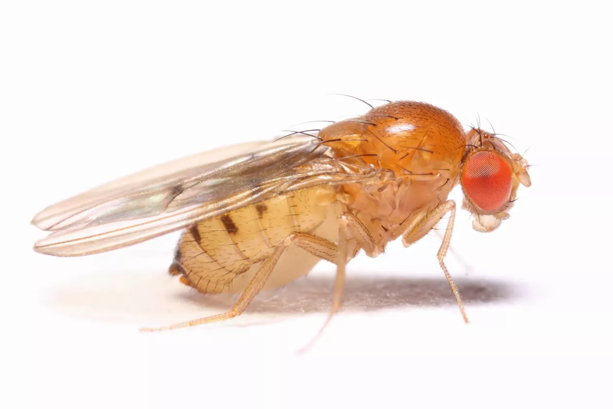
Drosphila melanogaster
In her study of fruit flies, Dr. Virginia Walker mated a bunch of homozygous wild type (WW) males to females with a brown eye recessive maker (bb). She then let the offspring mate with one another and scored the eye colours in the F2 generation. If the inheritance of eye colour is Mendelian, the expected distribution of genotypes for eye colour is 1:2:1 (WW:Wb:bb) but since WW and WB individuals both have red eyes, the expected ratio of eye colours is 3 red: 1 brown. By genetic analysis, she was able to determine the actual genotypes of all the F@ generation. She found that the ratio of eye colours was 224:72 (expected ratio is 3:1) and the ratio of genotypes was 56:168:72 (expected ratio is 1:2:1). She performed chi-square goodness-of-fit tests on these two observed distributions and found, for eye colour that chi-square = 0.07, P = 0.79 and for the genotypes that chi-square = 7.14, P = 0.03.
Considering that P≤0.05 is considered to indicate statistical significance we can conclude from these analyses that the distribution of eye colours is not significantly different from the expected distribution based on Mendelian inheritance but the distribution of genotypes is significantly different from the expected distribution so maybe there isn't Mendelian inheritance of this trait after all.
Contingency Table Analysis
Sometimes we count things rather than measuring them. For example we might be interested in the association between two variables, and can study this association simply by counting the number of individuals in each category. The result is a contingency table that looks like this:
This table shows the number of undergraduate courses that have male-, female- and equal sex ratios of students. The question we are interested in is whether the sex ratio in a course varies across disciplines—i.e. is sex ratio contingent upon discipline. In this sort of analysis it is usual to ask which variable is the cause (discipline here) and which is the effect (sex ratio here) but that does not affect the analysis, just the interpretation. Obviously, in this case, the discipline does not result from the sex ratio.
To run a contingency table analysis, construct a table like the one above (you can have as many rows and columns as you want but fewer is usual better, combining categories with small numbers if possible. Then enter you data in one of the on-line tables for analysis:
- Vassar Stats: enter data for up to 5 rows and 5 columns; lots of interesting output, explained.
- Quantpsy page: enter data for up to 10 rows and 10 columns; excellent instructions, warnings and explanations.
- Physics stats: enter up to 9 rows and 9 columns; uses several steps to build you and analyse your table; gives expected values and basic chi-square stats.
- SISA stats: an excellent analysis with lots of interesting output and graphs but data entry and choices are more complex than the others.
Sometimes it is best to run the Fisher exact test when you have a 2×2 contingency table, and here are some sites for that:
- GraphPad Stats: excellent explanations and analyses.
- SISA FISHER: excellent but complex output.
- Vassar Fisher: simple test, simple output.
Whatever analysis you perform, check to make sure you have satisfied the assumptions. Interpret the P-value as indicating (P≤0.05) a significant association between the two variables, or not suggesting an association (P>0.05).
A Worked Example
Dr. John Smol wants to know if there is an association between the pH of lakes and the presence/absence of 3 species of Daphnia. He has categorised each of 40 lakes in northern Ontario as high or low pH and then sampled to see which species were present. He found:
The analysis gave: chi-square = 6.11 (Yates correction for continuity), P = 0.01. This there is a significant association between Daphnia species and lake pH, though further analysis would be needed to determine which species are different in their response to pH. That could be done with a series of 2×2 contingency table analyses.
Assessing Normality
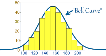
The Bell Curve is a normal distribution
Many of the statistical tests we are interested in assume that the data are sampled from a population where the variable of interest is normally distributed (Gaussian). It is usually a good idea to at least examine a plot of the data to see if it appears to be normally distributed, and if it isn't to transform the data appropriately.
The simplest plot that can be used to assess the fit to normality is a histogram. This one looks approximately normal because it is more or less bell-shaped:
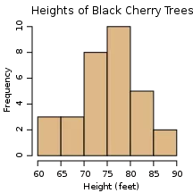
Approximately normal distribution
Whereas this one is quite skewed to the right:
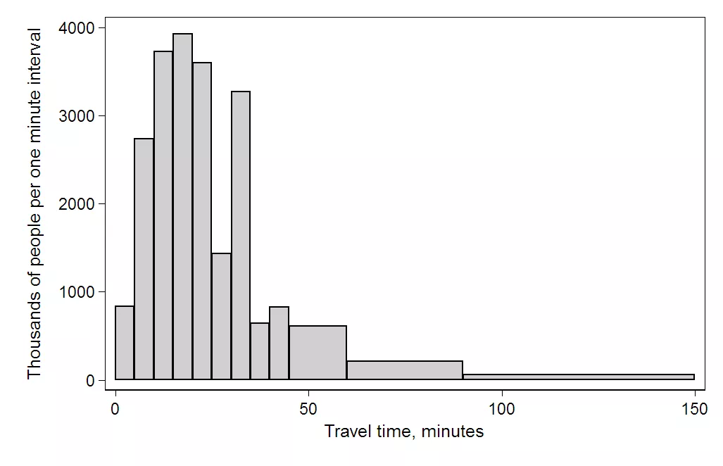
A right (or positive) skewed distribution
There are more formal statistical tests of normality (like the Shapiro-Wilk test) but in practice these are usually too stringent for most problems, and are thus more likely than they need to be to find that your distribution is significantly different from normal.